HPC-Accelerated Music Recommender

Overview

Given ~120K users and ~5.6M unique tracks, materializing the full user-track ratings matrix is infeasible (~670 billion entries, of which only a small fraction carry signal). Matrix factorization instead approximates this matrix as the product of two compact (low rank) embedding matrices, U (users × k) and S (tracks × k), which explain observed listening behavior, and can be used to generalize to unobserved behavior (inference time).

For training, Alternating Least Squares (ALS) is used on implicit feedback (play counts converted to a binary preference and a logarithmic confidence weight). Both the user step and item step are embarrassingly parallel, a natural fit for GPU batched solves, and the primary reason I chose a MF model for this project. Inference consists of a simple dot product and top-K sort, which is implemented through a single large SGEMM plus a parallel top-K in the GPU accelerated path, exactly the dense linear algebra cuBLAS is built for.

Approach

• Low-rank factorization. Replace the sparse 120K × 5.6M ratings matrix with two dense embedding matrices U ∈ ℝ^120K×64 and S ∈ ℝ^5.6M×64. The predicted preference for user u on track i is simply the dot product of the respective rows.
• ALS with implicit feedback. Each ALS sub-problem has a closed-form solution: U_u = (S^TC^uS + λI)⁻¹S^TC^up^u. Loss decreases monotonically and convergence is guaranteed.
• The computational trick. S^TC^uS decomposes into a constant term S^TS (computed once per iteration) plus a sparse correction over only the tracks user u actually listened to - reducing each user update from O(n) to O(n_u), where n_u is typically 50–500 instead of all n = 5.6M tracks.
• Batched GPU solves. The per-user k×k linear systems are batched into cublasSgetrfBatched + cublasSgetrsBatched calls (chunked across users to stay within GPU memory), saturating the GPU's arithmetic units.
• Inference at scale. A batch of 1000 concurrent requests becomes one cuBLAS SGEMM of shape (1000 × 64) · (64 × 5.6M) - about 720 billion floating-point operations - completed in milliseconds, followed by a parallel top-K argpartition kernel. A Python script is used to simulate request/response model, rather than a full backend implementation.

Pipeline

1. Preprocessing (Python). Chunk-reads 1B+ listening events, filters low-signal users/tracks, re-indexes to dense IDs, splits per-user train/val, writes .npz arrays.
2. CPU training baseline (NumPy/SciPy). Single-threaded ALS reference - establishes correctness and a wall-clock baseline.
3. GPU training (CUDA + cuBLAS). Batched LU factorization and solve on the GPU for both the user step and the item step. Binary embedding matrices written for inference.
4. CPU inference baseline (C++ + OpenBLAS + OpenMP). Parameterizable threading - serves as the non-HPC and HPC-CPU reference for the latency comparison.
5. GPU inference (CUDA + cuBLAS). Embeddings loaded once into GPU memory, concurrent requests served via SGEMM + parallel top-K kernel.

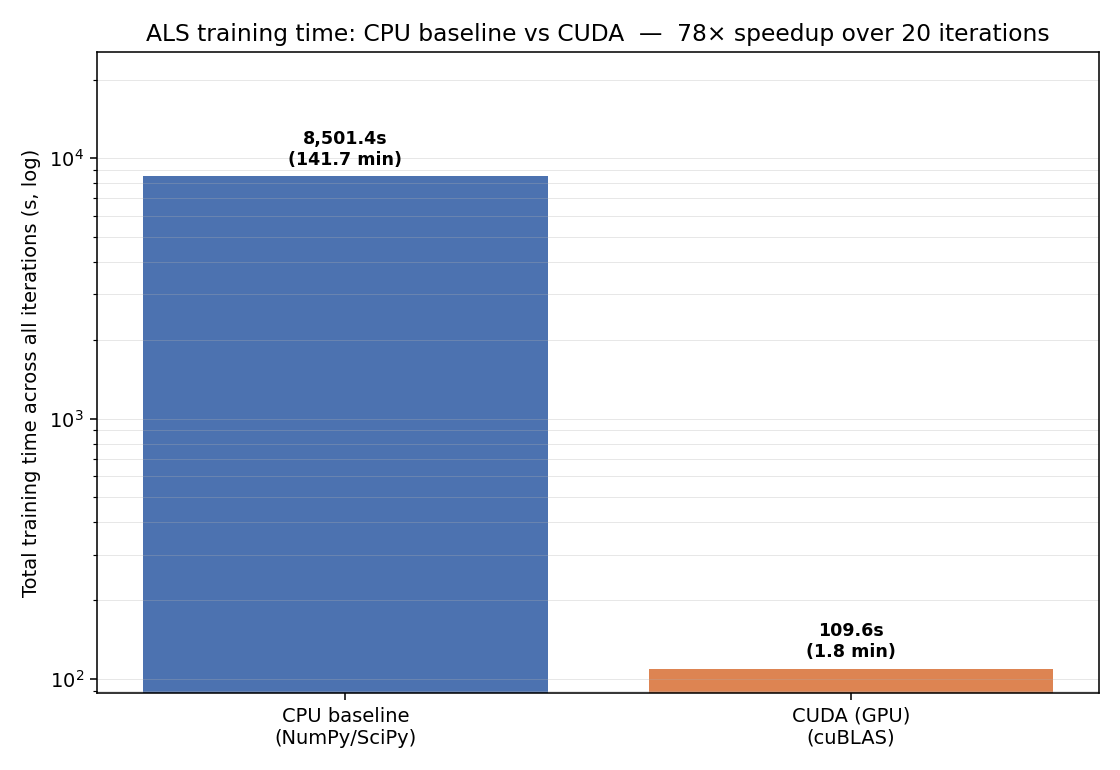
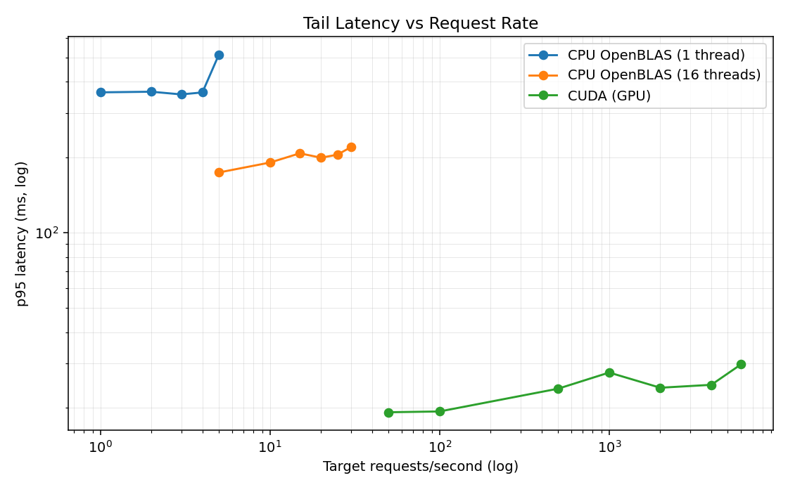
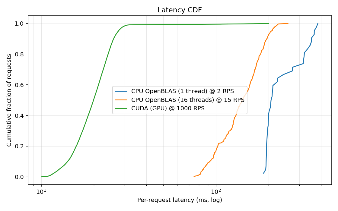
Results

The CPU baseline (single-threaded NumPy/SciPy or OpenBLAS+OpenMP) and the GPU build (CUDA + cuBLAS) are run on the same preprocessed data and benchmarked end-to-end - training wall-clock, request latency under load, and tail-latency scaling.